MUSE

Step-by-Step Guide: MUSE Data Reduction using EsoReflex

Last updated November 4, 2022.

This document is a brief step-by-step guide on using the MUSE pipeline on EsoReflex to perform standard data reduction. For further support, please contact the ESO Support using the webform available at https://support.eso.org.

Table of Contents

1. About MUSE Raw Data
   1.1. Downloading MUSE Raw Data
   1.2. Checking The Headers
   1.3. Dealing with (or without) SKY Data
   
2. Running EsoReflex and Setting Up for Standard Data Reduction MUSE Workflow
   
3. Co-adding / Combining Exposures
4. ZAP
5. Tips and Tricks
6. Citing EsoReflex and MUSE pipeline
7. References

1. About MUSE Raw Data

1.1. Downloading MUSE Raw Data

To download the raw data of any objects taken with MUSE, you could either use the ESO Observational Raw Data Query Form or the ESO Archive Science Portal. Either way, it will lead you to the Download Portal where you could do “run association” to look for the associated calibrations data. Finally, you could download the shell script to download all the files to your system (depending on the status of the data, proprietary or public, it will ask for your ESO User password). To run the shell script with 5 wgets in parallel and to circumvent interrupted download (to continue the partially-downloaded data from previous execution of the script, instead of re-downloading the same data), one can use:

  $ sh downloadScript_XXXXXX-XXXXX.sh -X "-n 1 -P 5" -d -c

The detailed description about the different type of MUSE data can be found in MUSE Pipeline User Manual chapter 5.

1.2. Checking The Headers

To display the FITS header information of your data, you can use the set of commands: dfits and fitsort. dfits will dump FITS headers as queried (e.g. using grep) and fitsort will sort the dfits output by a specified keyword. There is a Python module called dfitspy that does all of the dfits and fitsort capabilities. Below is an example of using dfitspy:

1. To display specific FITS headers values of all files in the directory:

      import dfitspy
   
      f = dfitspy.get_files(["all"])
      keys = ["OBJECT", "EXPTIME", "DATE-OBS", "HIERARCH ESO DPR CATG"]
   
      fitsort = dfitspy.dfitsort(f, keys)
      dfitspy.dfitsort_view(fitsort)
   

   Output:

   

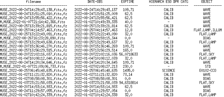
2. To display specific FITS headers values of files which “HIERARCH ESO DPR CATG” value is “SCIENCE”:

      fitsortgrep = dfitspy.dfitsort(f, ["OBJECT", "EXPTIME", "DATE-OBS", "HIERARCH ESO DPR CATG"], grepping=["SCIENCE])
      dfitspy.dfitsort_view(fitsortgrep)
   

   Output:

   

To perform dfits + fitsort commands using dfitspy module and write the output into a .csv file, see this Python script.

1.3. Dealing with (or without) SKY Data

The MUSE pipeline has two major ways to evaluate the sky to be subtracted from your target data:

• if the dedicated sky observations are present, the sky can be evaluated using a specified fraction of spaxels in the reconstructed sky image.
• or, the sky can be evaluated directly on your target data (frames), in a region where the contribution from the target is negligible. A user-specified fraction of spaxels in the reconstructed image will be selected to create the sky spectrum.

For most of the MUSE observations where sky observations are available, each Observing Blocks (OBs) would contain both the object and the sky exposures. More often than not, the sky observations require exposures way outside the object’s field of view, yielding to separate OBs from the object. If this is the case, in order to allow EsoReflex recognizes the respective sky exposures, they have to have the same values for the “HIERARCH ESO TPL START” headers. A custom python script for this purpose is available here (note that this script has to be placed in the parent directory of your RAW data directory!!).

2. Running EsoReflex and Setting Up for Standard Data Reduction MUSE Workflow

MUSE pipeline on EsoReflex processes individual exposures independently and, depending on your need, it could also align and combine exposures of the same object into one single final datacube. The below table contains the brief step-by-step guide on how to set up EsoReflex to do the standard data reduction on MUSE data (individual exposures independently).

#	Steps	Descriptions
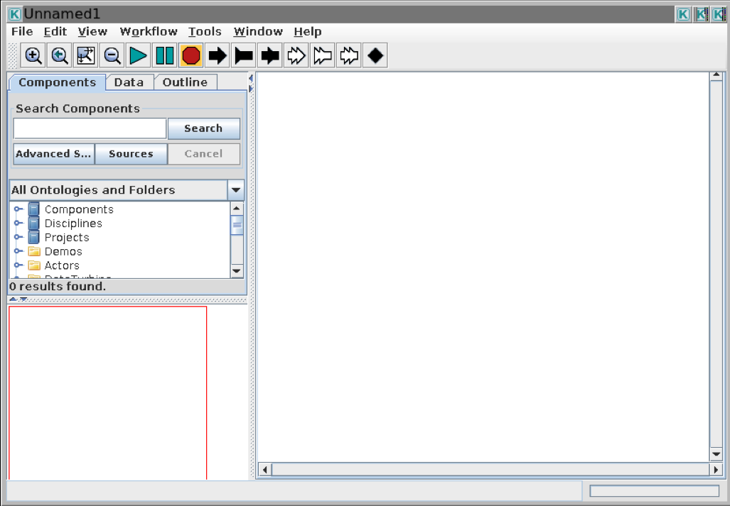
1.	Starting EsoReflex	Start EsoReflex from the terminal: $ install_dir/bin/esoreflex Or if you have a modified configuration file to use: $ install_dir/bin/esoreflex -config modified_esoreflex.rc Fig.1 - The empty EsoReflex canvas. More about the configuration file, esoreflex.rc, can be found in the EsoReflex User Manual section 8.2. (p.26).
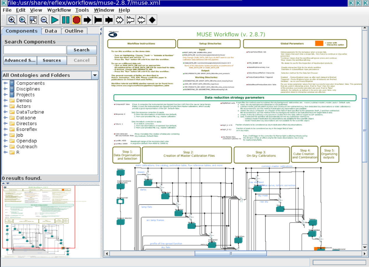
2.	Opening MUSE pipeline	On the menu bar, go to File - Open..., browse your MUSE pipeline (the latest version is 2.8.7) folder, and choose muse.xml. It will open a new window of the MUSE pipeline workflow. Fig.2 - The MUSE pipeline workflow. Navigating on the EsoReflex canvas can be tricky and unintuitive. ... More to come (on the navigating the EsoReflex canvas)...
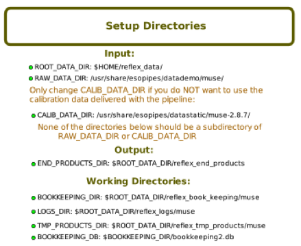
3.	Setup Directories	You would need to adjust the ROOT_DATA_DIR and RAW_DATA_DIR to your working directory and the directory where your raw data are located, respectively. Leave the CALIB_DATA_DIR as is. To edit, double click on the words and then browse the proper directory. Fig.3 - The default Setup Directories.
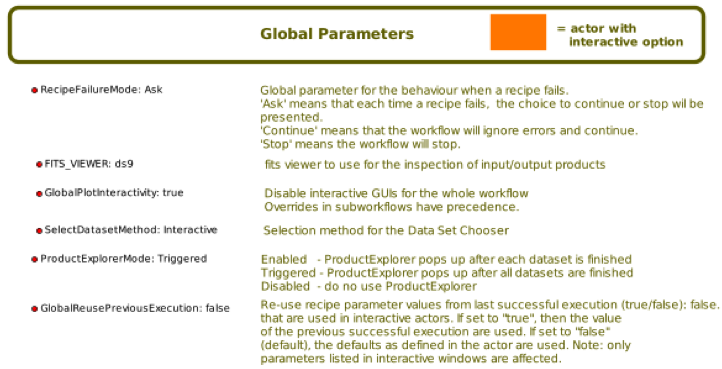
4.	Global Parameters	I usually leave everything here as default. But, it would be quite a time-saving to change RecipeFailureMode from the default "Ask" to "Continue" which tells the workflow to ignore any errors and/or exceptions. Do this at your own risk. Fig.4 - The default Global Parameters.
5.	Data Reduction Strategy Parameters	The parameters that I commonly change: LamMin and LamMax: 4750 - 9350 (the default values are 4000 and 10000). The useful wavelength (is defined by the range for which the MUSE field of view is fully sampled) for the nominal mode is 4750 - 9350 Angstrom and for the extended mode is 4600 - 9350 Angstrom. SkyMethod: this value depends on the data you are working on (the available options: none, subtract-model, model, simple, auto; detailed description about each option are available on the workflow window or in the EsoReflex MUSE Tutorial p.26), MUSE pipeline has two major ways to evaluate the sky to be subtracted from your target data: if the dedicated sky observations are present, the sky can be evaluated using a specified fraction of spaxels in the reconstructed sky image. This fraction is specified by the SkyFr_1 parameter on the workflow (set SkyMethod parameter to subtract-model) or, the sky can be evaluated directly on your target data (frames), in region where the contribution from the target is negligible. A specified fraction of spaxels in the reconstructed image will be selected to create the sky spectrum, this is the SkyFr_2 parameter on the workflow (set SkyMethod parameter to model and in this case, the SkyFr_1 has no effect) Use Raman lines correction?: if you are working with MUSE AO data, this field needs to be "yes". Observations using the adaptive optics are affected by Raman scattered light from the Na lasers. This contamination varies slowly across the field (+/- 5%) and shows up mainly as emission lines at 6485 Angstrom and 6827 Angstrom. The majority of this contamination is taken care of during the sky subtraction process (where Raman lines get reduced down to about 5%), however the correction procedure reduces the Raman line fluxes to < 1%, which works best for observations of nearly empty fields. Important notes: The correction is efficient only if large part of the FoV of the target is dominated by sky. It is not recommended for the NFM data. If it is applied to the densely populated FoV data, it may create artifacts and compromise the correction. If it is enabled for the observations with dedicated sky frames, the correction removes the Raman contamination twice. More about this can be read on the EsoReflex MUSE Tutorial p.27-28 or on the MUSE Pipeline User Manual Sect. 6.5.4. Fig.5 - The default Data Reduction Strategy Parameters.
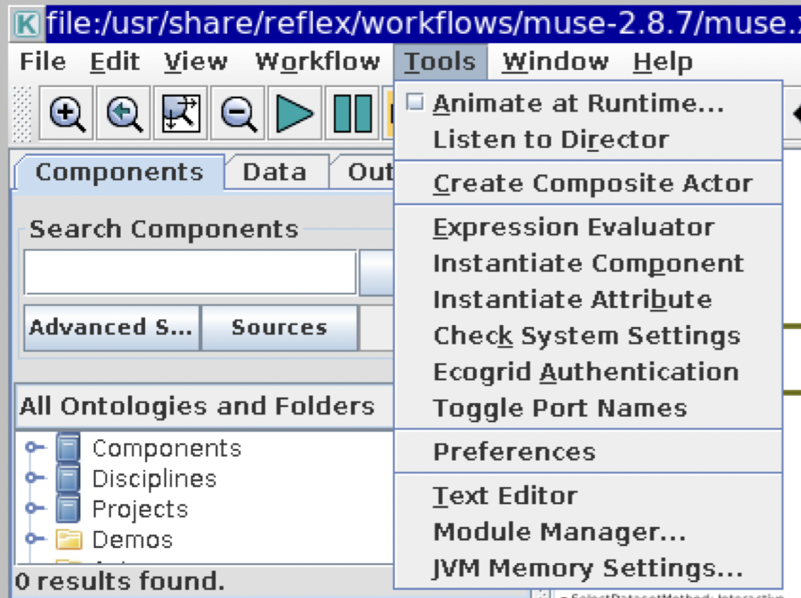
6.	Animate at Runtime	Tools - Animate at Runtime..., turn it on to aid in the visual tracking (the folder, or an actor, at which the workflow is currently at will be highlighted with red) of the reduction cascade (100 ms is recommended for the animation interval). Fig.6 - The Tools dropdown menu. For a more comprehensive explanation of each parameter and each actor in the MUSE workflow, please see the EsoReflex MUSE Tutorial.
7.	Running the workflow	Run the workflow by clicking the Run button (the highlighted button on Fig.7 below) on the top bar. Fig.7 - The Run button.
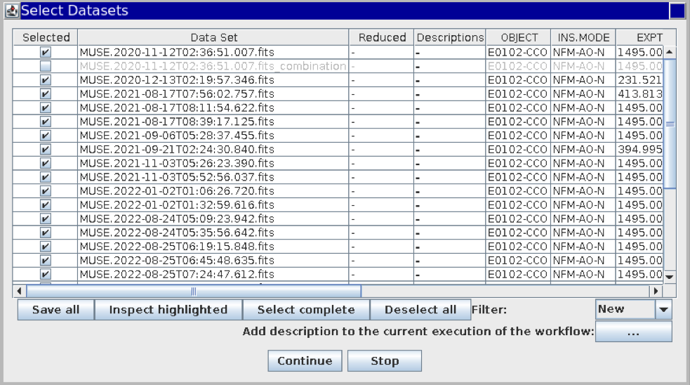
8.	Select Datasets	The Select Datasets table will pop up once the workflow reaches the Exposure Selection actor. It is an interactive window which lists the datasets with the values of select header keywords. The first column consists of a set of tick boxes that allow the user to select the datasets to be processed. Fig.8 - The Select Datasets pop-up window.
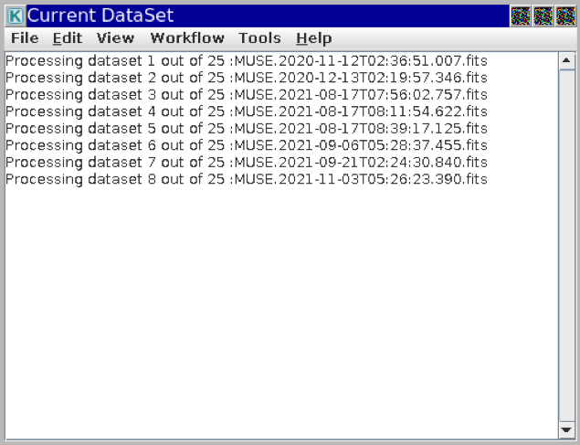
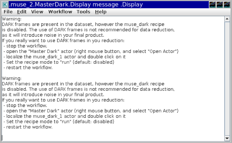
9.	Pop-up windows during the run	During the run, there will be several pop-up windows with information regarding the datasets. The common ones (and will always be there) are the Current DataSet and Finished Datasets windows. There will also be some warning messages or error messages (see [Possible Error and Exception Messages](#error) in [Section 5](#tips)). Fig.9 - The Current DataSet pop-up window. Fig.10 - The Finished Datasets pop-up window. Fig.11 - An example of warning or error message pop-up window.
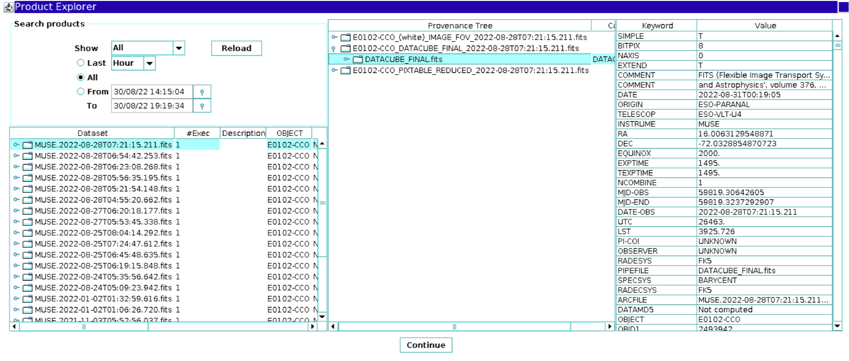
10.	Product Explorer	Once the data reduction workflow is finished, a Product Explorer window will show up. It shows the final products and allows the users to inspect the datasets. To close the window and to finish the run, click the "Continue" button. Fig.12 - The Product Explorer window.

3. Co-adding / Combining Exposures

After doing the standard data reduction on each dataset, user could choose to combine all of them into a single datacube, using the same muse.xml file. Before proceeding, make sure that the values of HIERARCH ESO OBJ TARG NAME and HIERARCH ESO INS MODE headers for all exposures are the same (see EsoReflex MUSE Tutorial p.20 for more details).

#	Steps	Descriptions
1.	Starting EsoReflex and Opening the MUSE pipeline	Run EsoReflex normally and open the muse.xml.
2.	Setup Directories	Update ROOT_DATA_DIR and RAW_DATA_DIR in the Setup Directories to the directories where you want the end products to be saved at (including the temporary data) and where your reduced datasets are located.
3.	Running the workflow	Run the workflow by clicking the Run button (see Fig.7) on the top bar.
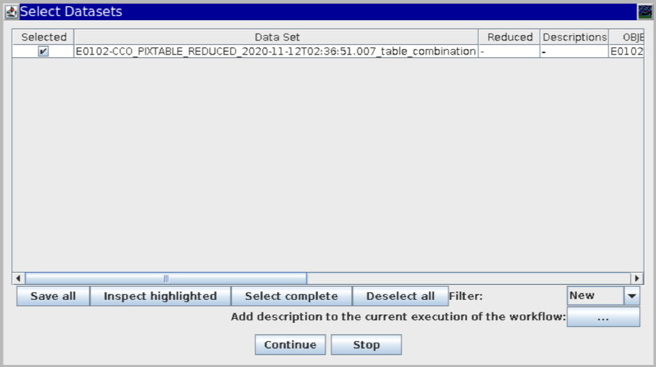
4.	Exposure Selection	The Select Datasets table will pop up once the workflow reaches the Exposure Selection actor. In this case, the Data Set column will show all the reduced PIXTABLEs available. Fig.13 - The Select Datasets window for the exposure combination. You could select the datasets you want to use in the combination by clicking on the line item to highlight it, then click "Inspect highlighted" button. Fig.14 - The Select Frames window.
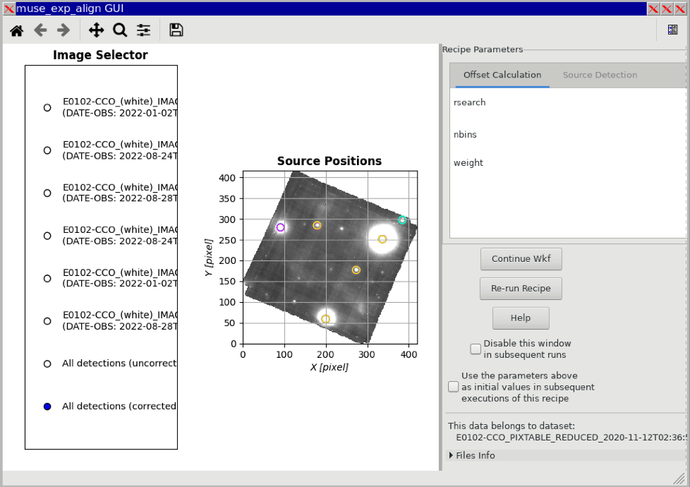
5.	Image Selector	muse_exp_align GUI will show up and you are able to inspect each dataset. If you are satisfy with the alignment, you can continue with clicking the "Continue Wkf" button to resume the workflow and run the "CombineExposures" actor. Fig.15 - The Image Selector window.
6.	Product Explorer	Once it is done, the Product Explorer window (see Fig.12) will pop up.

4. ZAP

… More to come…

Create Datacube with sky residual parameter has to be set to true.

5. Tips and Tricks

Most of these are coming from personal experience.

Arranging your directories

• Make sure that the ROOT_DATA_DIR is not located within the same parent directory as

… More to come…

Closing a long-as* pop-up window

… More to come…

Terminating the workflow

… More to come (to stop the process)…

Saving the Kar

… More to come…

Possible Error and Exception Messages

Exception on the start of the Data Organizer actor.

• Cause: incomplete download of the raw data or corrupt file(s) in the raw data directory.
• Solution: remove the corrupt file, if you know which one or re-download your raw datasets.

Fig.16 - An exception that might occur on the Data Organizer actor stage.

Error on esorex.log file does not exist.

• Cause: .
• Solution: So far, it seems that it does not affect much of the workflow, when "Continue" chosen, the workflow proceeded until the end.

Error on “Missing required sky lines frame for sky model”.

• Cause: Raman scattering correction (this needs confirmation from the ESO Support).
• Solution: Set to no, for now.

6. Citing EsoReflex and MUSE pipeline

Acknowledge EsoReflex by citing the Freudling et al. 2013 paper (BibTeX entry) and the MUSE pipeline by citing the Weilbacher et al. 2020 paper (BibTeX entry) and its ASCL (BibTeX entry).

References

The MUSE second-generation VLT instrument, Bacon, R., Accardo, M., Adjali, L., et al. 2010, SPIE, 7735, 773508.
Automated Data Reduction Workflows for Astronomy: The ESO Reflex Environment, Freudling, W., Romaniello, M., Bramich, D. M., et al. 2013a, A&A, 559, A96.
The data processing pipeline for the MUSE instrument, Weilbacher, P. M., Palsa, R., Streicher, O., et al. 2020, A&A, 641, A28.